



Section 1.5: Power and Measurements #
Having explored how impedance matching helps transfer power between components, we now need to understand how to measure and quantify this power.
Power Fundamentals #
At its most basic level, electrical power is the rate at which energy is transferred in a circuit:
Where:
- is power in watts (W)
- is current in amperes (A)
- is voltage (Electromotive force) in volts (V)
Replacing in with from Ohm’s law gives . Replacing with instead gives . That gives us three equivalent forms:
These equations let us calculate power in a resistive load when we know at least two of the following: voltage, current, or resistance. AC circuits containing reactance also require attention to the phase relationship between voltage and current.
For example:
- With 12 volts and 0.2 amperes:
- With 7 milliamperes through 1,250 ohms:
If we apply 400 VDC to an 800-ohm load, we can calculate the power:
AC Power and RMS Measurements #
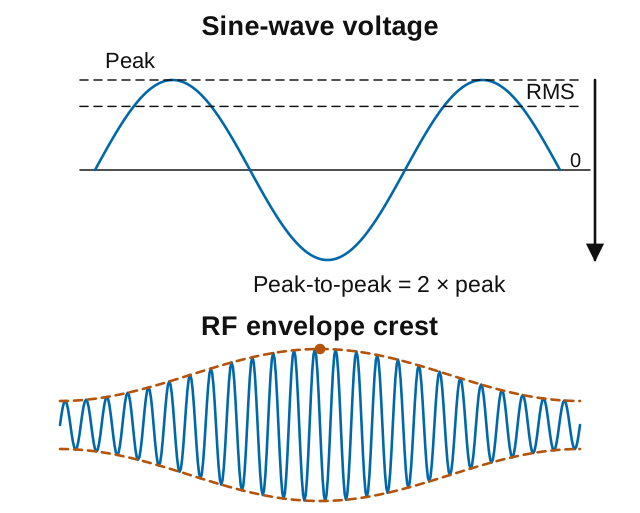
With alternating current, voltage and current constantly change. For a sine wave centered on zero, the positive and negative halves cancel when we average its voltage. The result is zero. So how do we apply Ohm’s Law and power formulas to AC circuits?
The answer is Root Mean Square (RMS) values. RMS is a special mathematical method that gives us an effective value for AC that works in our DC-based equations:
Key Information: The RMS value of an AC signal produces the same power dissipation in a resistor as a DC voltage of the same value.
Why use RMS instead of averaging the absolute values—the voltage readings without their minus signs? It’s because of how power works in resistive circuits. Power is proportional to voltage squared ( ), not to voltage directly. The heating effect in a resistor—which is what actually matters in power calculations—depends on this squared relationship.
If we used the average of absolute values, our power calculations would be incorrect. Though not needed for the exam, it’s useful to know that RMS accounts for this squared relationship between voltage and power by:
- Taking the square of each instantaneous value (the “Square” in RMS)
- Finding the average (Mean) of those squared values
- Taking the square Root of that average
For a sine wave, this works out to:
For a resistor, using RMS voltage in gives the average power dissipated as heat. When you hear that household electricity is 120 volts, that’s the RMS value, not the roughly 170-volt peak of its sine wave.
For example:
- If you have 17 volts peak AC, the RMS voltage is:
- If you have 120 volts RMS AC, the peak-to-peak voltage is:
We can also calculate RMS voltage from power measurements:
- With a 50-ohm load dissipating 1200 watts:
The following table shows the relationships between voltage measurements for a sine wave:
| Measure | Relationship to RMS |
|---|---|
| RMS | (reference) |
| Peak | |
| Peak-to-Peak |
RF Power Measurements: PEP #
When you transmit voice or other complex signals, RF power can vary moment by moment, depending on what you send. We need a consistent measure. Peak Envelope Power (PEP) provides that standard, helping us follow the rules and avoid damaging equipment.
PEP is the average power over one RF cycle at the crest of the modulation envelope. The envelope follows the slower changes in the RF signal’s amplitude, such as the peaks of speech. PEP describes those envelope peaks, not the highest instantaneous power within a single RF cycle. That distinction lets us compare changing signals using a consistent power measurement.
Key Information: For an unmodulated carrier, the ratio of PEP to average power is 1.00, meaning that the PEP and average power are the same.
For a continuous carrier with no modulation (like a test tone or CW signal with the key down), PEP equals the average power because the power level remains constant. But with voice modulation, especially on SSB, the power output spikes during louder syllables. These momentary peaks might be several times higher than the average power level.
For a sine-wave RF signal across a resistive load, using the peak RF voltage at the envelope crest gives:
When working with peak-to-peak voltage measurements, this becomes:
For example:
- With 200 volts peak-to-peak across 50 ohms:
- With 500 volts peak-to-peak across 50 ohms:
Logarithmic Measurements: Decibels #
Radio science frequently uses decibels (dB) because they simplify how we express large changes in power. Instead of saying a signal has “100 times the power,” we can say it’s “20 dB stronger.” This makes calculations easier and allows us to add gains and losses instead of multiplying and dividing.
Key Information:
- An increase of about 3 dB doubles power; a decrease of about 3 dB halves power.
- A loss of 1 dB represents a power loss of approximately 20.6 percent.
Positive dB values represent power increases, while negative dB values represent decreases. Here are useful approximate power ratios to remember:
| dB | Power Ratio | Description |
|---|---|---|
| 1 dB | 1.26 | 26% increase |
| 2 dB | 1.58 | 58% increase |
| 3 dB | 2 | 2x power |
| -3 dB | 0.5 | power |
| 6 dB | 4 | 4x power |
| 9 dB | 8 | 8x power |
| 10 dB | 10 | 10x power |
| 20 dB | 100 | 100x power |
| 30 dB | 1000 | 1000x power |
Note: For a power decrease, take the reciprocal of the corresponding positive-dB ratio. For a 3 dB loss, start with the +3 dB ratio of 2: half the power remains. If that positive-dB ratio is , the fraction lost is ; multiply by 100 to express the loss as a percentage. For example:
- -3 dB:
- -1 dB:
Decibels in Radio Applications #
The decibel’s flexibility makes it ideal for several specialized radio measurements:
Antenna Gain Measurements #
Key Information: Antenna gain expressed in dBi is 2.15 dB higher than the same gain expressed in dBd.
Two common reference points for antenna gain are:
- dBi: Gain compared to an isotropic radiator, an ideal source that radiates equally in every direction
- dBd: Gain compared to a half-wave dipole in free space
That reference dipole has about 2.15 dBi gain. We can therefore express an antenna’s 6 dBd gain as 8.15 dBi. The antenna has not changed—only the reference has.
Accounting for Losses #
Decibels also describe power that fails to reach its destination. Suppose your transmitter delivers 100 watts and the feed line loses 3 dB before the antenna. About half the power, or 50 watts, reaches the antenna. If another component introduces another 3 dB loss, about 25 watts remain. The losses add to 6 dB, while the power is halved twice.
That is why a power increase at the transmitter does not necessarily produce the same power at the antenna. Section 4.1 applies this accounting to actual feed lines and their loss specifications. For now, the useful tool is the relationship between a dB change and the corresponding power ratio.
Exam Questions #
At most one of the questions in this table can appear on your exam.
| Question | Equation | Answer |
|---|---|---|
| G5B01: dB change for 2x power increase/decrease | dB | 3 dB |
| G5B03: Power with 400 VDC and 800 ohms | ||
| G5B04: Power with 12V and 0.2 amperes | ||
| G5B05: Power with 7mA and 1,250 ohms | ||
| G5B06: PEP with 200V peak-to-peak across 50 ohms | ||
| G5B08: Peak-to-peak voltage from 120V RMS | ||
| G5B09: RMS voltage from 17V peak | ||
| G5B10: Power loss from 1 dB | 20.6% | |
| G5B11: PEP to average ratio for unmodulated carrier | 1.00 | |
| G5B12: RMS voltage with 1200W across 50 ohms | ||
| G5B13: PEP of unmodulated carrier with 1060W average | PEP = Average Power (for unmodulated carrier) | |
| G5B14: PEP with 500V peak-to-peak across 50 ohms |
You can learn the calculation methods or memorize these answers for now. Return to the worked examples when you need to apply the math.
Moving Forward #
These principles will serve as the foundation for evaluating transmitter performance, understanding receiver sensitivity, and optimizing antenna systems as we continue through the book. In the next chapter, we’ll build on this knowledge as we explore the components that make up amateur radio circuits.



 2.4 watts