Section 6.8: Reading the Smith Chart #

The stub at the end of the previous section needs two numbers: its distance $d$ from the antenna and its length $\ell$ . Both depend on how impedance changes along the line, and calculating that change point by point is slow. On a Smith chart, each point represents one complex impedance, $R+jX$ , and moving along a line moves that point in a predictable way. At first glance, the chart looks like a tangle of circles. Learn its two families of curves, and the tangle becomes a map.

Key Information: Impedance along transmission lines can be calculated using a Smith chart.

Two Families of Curves #

On the rectangular impedance plot from Section 2.2, resistance runs horizontally and reactance vertically. A Smith chart bends those coordinates into circles and arcs. Select one resistance circle and one reactance arc; where they cross marks the impedance.

Figure E9-3, a normalized impedance Smith chart. A horizontal resistance axis runs from zero at the left edge through one at the center to infinity at the right edge. Constant-resistance circles touch the right edge and cross the horizontal axis at their labeled values, including 0.2, 0.5, 1, 2, and 5. Constant-reactance arcs run from the large outer circle toward the right edge. The upper half represents positive inductive reactance and the lower half negative capacitive reactance; the printed arc labels give magnitudes. The center represents a resistive load equal to the chosen reference impedance. No wavelength scales or added constant-SWR circles are shown in this simplified figure. — Figure E9-3: Resistance circles and reactance arcs.

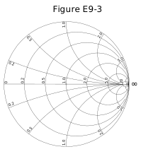
Resistance labels lie along the horizontal diameter; each names the complete circle that crosses the diameter there. Every resistance circle touches the right-hand edge. Reactance labels lie around the outer rim; each names an arc curving inward toward that same right-hand point. Positive, inductive reactance occupies the upper half and negative, capacitive reactance the lower half. The printed labels give only magnitudes, so location supplies the sign.

A constant-resistance circle does not have constant distance from the chart’s center. Follow the resistance circle labeled 1.0 at the center: its resistance stays 1 while its reactance changes. That distinction will matter when we add SWR circles.

Every point on the horizontal diameter has zero reactance; its left end is a short circuit and its right end an open circuit. Every point on the large outer circle has zero resistance.

Key Information:
A Smith chart uses a coordinate system of resistance circles and reactance arcs.
The two families of circles and arcs that make up a Smith chart are resistance and reactance.
The arcs on a Smith chart represent points with constant reactance.
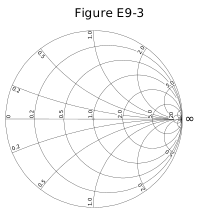
On the Smith chart shown in Figure E9-3, the only straight line shown is the resistance axis.
The large outer circle on which the reactance arcs terminate is the reactance axis.

Give the Center a Value #

The same printed chart can serve a 50-ohm coax system or a line with another impedance. Normalization makes that possible: divide every impedance by the chosen reference $Z_0$ . The chart’s center point is called the prime center. Marked 1, it represents a resistance equal to $Z_0$ and zero reactance.

Key Information: A Smith chart is normalized by reassigning the prime center’s impedance value.

For a 50-ohm system, divide $100+j50\ \Omega$ by 50. The result is $2+j1$ . Find the resistance-2 circle and the positive-reactance-1 arc; their upper-half intersection represents the load. Multiply the chart values by 50 to return to ohms. If the reference were 75 ohms, the same chart point would mean $150+j75\ \Omega$ .

A Smith chart with a faint grid. The horizontal diameter is drawn dark and labeled resistance axis, with short at its left end and open at its right end. The dark outer circle is labeled reactance axis. A dot at the center is labeled prime center, 1. One resistance circle, labeled r equals 2, is drawn heavy in blue; it touches the right-hand end and crosses the axis to the right of center. One reactance arc, labeled x equals plus 1, is drawn heavy in orange; it runs from the top of the rim down to the right-hand end. Where the circle and arc cross, in the upper half, a dot is labeled 2 plus j1. Text at the upper left reads plus jX inductive, and at the lower left minus jX capacitive. — Reading the chart: r and x are normalized resistance and reactance. The resistance-2 circle and the reactance +1 arc cross at 2 + j1, which is 100 + j50 Ω on a 50-ohm chart.

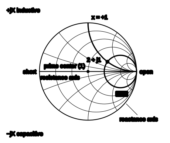
At the center, $1+j0$ means a perfect match to the reference. A point’s distance from the center represents the magnitude of its reflection coefficient. SWR depends only on that magnitude, as Section 6.3 showed, so points equally far from the center have the same SWR, even when their resistance and reactance differ.

Following a Transmission Line #

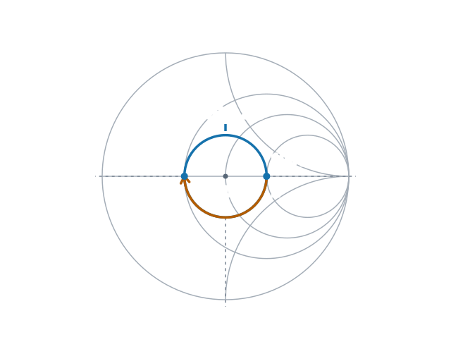
To find what impedance the transmitter sees through a length of line, start at the load point. Draw a circle through it, centered on the prime center. Moving along an ideal lossless line changes reflection phase but not magnitude, so the impedance moves around that circle while SWR stays constant.

A full working chart prints two wavelength scales around its rim, each running from zero to one-half wavelength; Figure E9-3 leaves them out. The scale for movement toward the generator, the transmitter end, increases clockwise. The scale toward the load increases counterclockwise. Both start from zero at the left, short-circuit end, so read the scale at the starting and ending points and take the difference. A full revolution covers one-half wavelength of line, because a reflection accumulates phase on both the outward and return paths.

For a 100-ohm load on 50-ohm line, the normalized load is 2, on the horizontal axis to the right of center. Where the constant-SWR circle crosses the horizontal axis to the right of center, the normalized resistance equals the SWR. Here it crosses at 2, giving 2:1 SWR. Move one-quarter wavelength toward the generator: that is half a turn around the constant-SWR circle. The new point is 0.5, or 25 ohms, the same quarter-wave inversion the Q-section in the previous section used. Another quarter wavelength brings you back to 100 ohms. Impedance changes; the lossless line’s SWR does not.

The heavy constant-SWR circle cuts across the faint resistance circles and reactance arcs. Its right-axis crossing at normalized resistance 2 gives 2:1 SWR. The arrow and rim marks measure movement toward the generator from this 100-ohm load: a quarter wavelength transforms it to 25 ohms.

Key Information:
Impedance and SWR values in transmission lines are often determined using a Smith chart.
Constant-SWR circles are the third family of circles often added to a Smith chart during the process of designing impedance matching networks.
The wavelength scales on a Smith chart are calibrated in fractions of transmission line electrical wavelength.

Placing a Matching Stub #

A stub connects in parallel, so the stub problem is easier with admittance, the reciprocal of impedance from Section 2.3. Parallel admittances add directly. Half a turn inverts a normalized impedance, as 2 became 0.5 above, so the point directly across the center from any impedance gives its normalized admittance. Working with those opposite points, move along the line to a junction where the real part is 1. A stub there can cancel the remaining imaginary part.

Key Information: A common use for a Smith chart is to determine the length and position of an impedance matching stub.

Suppose the main line’s admittance at the chosen junction is $0.02+j0.02$ siemens, or $1+j1$ normalized to 50 ohms. Its real part is already right: once the stub cancels the $+j0.02$ susceptance, 0.02 siemens alone is $1/0.02=50\ \Omega$ .

A shorted one-eighth-wave stub of 50-ohm line presents $+j50\ \Omega$ , so its admittance is $1/(j50)=-j0.02$ siemens, the same sign flip as in Section 2.3. Connected in parallel, the imaginary parts cancel and leave a 50-ohm resistive input.

With the electrical lengths in hand, find each one’s free-space length and multiply it by the line’s velocity factor. The result is the length of cable to cut. Measure twice; coax doesn’t grow back.